Environmental changes are posing a serious threat to production and nutritional value of our crops. Not taking action could have major global implications for food security and public health, a new study outlines.
A new study has further revealed how climate change is reducing
yields and sucking the nutrients from our vegetables and legumes,
raising serious questions over the future of food security and public
health around the world.
The report, which was led by the London School of Hygiene and Tropical Medicine,
is apparently the first of its kind to methodically examine to what
extent environmental changes such as water scarcity, increases in
temperature and a greater concentration of carbon dioxide could impact
the nutritional quality and yield of crops vital to our everyday
nutrition.
Previous
research into the impact of environmental change on food has mostly
focused on the yield of staple crops such as wheat, rice and corn.
However, there has been comparatively little discussion on how climate
change is affecting nutritious foods that are considered more important
to a healthy diet.
Vegetables scorched by a heat wave in China — such events may become more common in the future due to climate change
The 'junk food effect'
The phenomenon of
crops being stripped of their high nutritional qualities due to
environmental factors has become known as the "junk food effect."
For
some time now, researchers have been aware that many of our most
important plant-based foods are becoming less nutritious. Studies have
shown how the mineral, protein and vitamin content in fruits and vegetables has decreased over the past few decades, although until recently this had been explained away by the fact that we had been prioritizing higher yields over nutrition.
"Vegetables
and legumes are vital components of a healthy, balanced and sustainable
diet, and nutritional guidelines consistently advise people to
incorporate more vegetables and legumes into their diet," says lead
author Pauline Scheelbeek.
"However, our new analysis suggests
that this advice conflicts with the potential impacts of environmental
changes that will decrease the availability of these crops."
The carbon dioxide factor
Alongside
water scarcity and increasing temperatures, higher levels of carbon
dioxide are being blamed for stripping crops of their nutritional value.
But
carbon dioxide is good for plants, so why should we be worried about
rising CO2 levels? While it's true that plants do require carbon dioxide
in order to grow and thrive, it's possible to have too much of a good
thing.
Rising carbon dioxide levels ramp up the process of
photosynthesis — which is what allows plants to transform sunlight into
food. While this certainly helps plants grow, it has the side effect of
causing them to produce more simple carbohydrates such as glucose.
And this comes at the expense of other important nutrients we need in order to stay healthy including protein, zinc and iron.
The future of farming in a warming world
Food security a growing concern
The latest findings, published in Nature,
have alarming implications for food security and raise some
disconcerting questions about the future of our planet's food supply.
Hotter regions such as Southern Europe, Africa and South Asia are most at risk, where higher temperatures are already expected to reduce crop yields by about 31 percent.
But Scheelbeek says the total crop yield is not necessarily the most important factor to consider.
"I
think we have shifted from food intake being the biggest problem in
terms of global food security to the issue of nutrition," she told DW.
We currently grow far too many grains, say some experts
Tim Benton, a visiting fellow at Chatham House and a specialist in
food security and sustainability, agrees that the issue of food security
— at least from a global perspective — needs to be looked at through
the lens of public health and nutrition rather than focusing on the
amount of crops that we grow.
"It's a developed world problem and
a developing world problem," he told DW. Benton, who was not involved
in the new study, doesn't see the world heading toward starvation due to
not being able to grow crops. "But we are going to be in a situation
where public health gets worse."
Potential for a nutritional crisis
The reduced nutritional quality of important crops could mark the beginning of a looming health crisis.
One
of the biggest concerns addressed by the report is the potential
increase of micronutrient deficiencies. Around 1.5 million deaths per
year are already linked to low vegetable intake, according to the Global Burden of Disease (GBD) study.
The worldwide per capita daily consumption of fruit and vegetables is
already from 20 to 50 percent below the minimum recommended levels.
A paper published in Nature in 2014 highlighted how increased levels of carbon dioxide could also impact the nutritional value of staple crops such as rice, wheat and soybeans.
But
Benton stresses that at this stage, we should be more worried about the
non-staples. A focus on cash crops is part of the problem, he added.
"We currently grow three times as much grain and about a third of the amount of fruit and vegetables that we need," he told DW.
A lack of veg? Benton says too much grains and not enough nutritious fruit and vegetables are cultivated worldwide
Scheelbeek says various issues need to be considered if the
consumption of legumes and vegetables drops as a result of environmental
changes.
"For example, what would people eat instead? What would
be their substitution for a less-available or more expensive legume on
the market? It's certainly something we need to address."
Adaptation key to crisis
Experts say the best way to alleviate the threat to crops in the future is to prioritize changes in agricultural production.
Benton believes looking toward growing new crop varieties is "absolutely necessary" if we wish to avoid a crisis.
Scheelbeek
says the results of the study represent a "business-as-usual scenario,"
assuming very little action is taken over the next few decades.
"We
hope of course that the [results] of this study are a bit of an
eye-opener, and that this is a gap that we need to bridge to make sure
that there is enough nutritious food until the end of the century."
Feeding the world of the future: is hydroponics the answer?
Tackling food insecurity with hydroponics
The challenge of feeding a planet that’s set to have 3 billion more people on it by 2050 - made even more acute by climate change as some parts of the planet become wetter, while others drier - means the pressure is on to find ways to feed the planet. So farming has to become more productive – and new areas to grow, especially in dry climates, must be found. One potential solution: hydroponics. MORE
With climate change and the associated warmer temperatures already altering the timings and patterns of bird
migrations, climate change-induced human migration is not far behind.
Estimates suggest that by 2050 there are likely to be between 25 million and 1 billion environmental migrants in the world, with a major proportion of these originating from low and lower-middle income countries.
South Asia
is particularly vulnerable to climate change. Nearly half of the
region’s population lives in areas that are projected to become moderate to severe climate hotspots by 2050. Unhealthy temperatures and variable precipitation patterns
have contributed to declines in agricultural production, productivity
and food security. Natural calamities such as floods, tsunamis and
earthquakes have increased the susceptibility of the region’s already
vulnerable population.
Migration has emerged as an important survival and adaptation strategy. In Bangladesh alone, 15 million people are expected to be displaced due to the environmental degradation of the country’s coastal zone. The bulk of forced climate-induced migration has involved the most vulnerable.
The major migration corridors
in South Asia are between Bangladesh–India, Afghanistan–Pakistan,
India–Pakistan and Nepal–India. In 2015, more than 85 per cent of migrants in South Asia
originated from other countries in the region. There are currently
about 3,230,025 and 810,172 migrants from Bangladesh and Nepal
respectively in India.
Pakistan has about 2,326,275 Afghani migrants. With current levels of
transboundary migration already high, it is difficult to decipher the
number of these who are climate-induced migrants. As such, climate
change has remained largely invisible in discussions about migration. Empirical evidence
suggests that environmental degradation is an important factor in
pushing migration, particularly in less developed countries. With
climate change already impacting the availability of water, food and
arable land in host countries, transboundary migration is expected to
trigger conflicts and exacerbate tensions. Migration also contributes to
ethnic tensions, discords, distrust and the demolition of social
capital.
For instance, many illegal Bangladeshi immigrants are seeking
employment in India. This is leading to rising Indian intolerance
towards Bangladeshis, especially in Assam and West Bengal. Tensions are
also brewing between Bangladeshi migrants and the ethnic Bodo group in
Assam. The presence of a large number of Afghan refugees
in Pakistan’s Khyber Pakhtunkhwa is seen by the Pakistani military as a
security risk that aggravates drug trafficking, smuggling and terrorist
activities. Following the 2015 earthquake in Nepal, agitation by the Madhesis (an ethnic group of Indian origin) in Nepal contributed to nation-wide political turmoil.
The presence of Nepali migrants in Bhutan and India, Sri Lankan
Tamils in India and Chakmas in Bangladesh have increased security issues
for these countries. South Asia is already considered the second most violent place on earth after Iraq. In 2016,
about 20 per cent of all conflicts in the world took place in this
volatile region and resulted in about 22 per cent of total
conflict-related deaths. Climate-induced migration will worsen these
existing tensions.
Cross-border migration also impacts the psyche of migrants. For
instance, Pakistan has often used pressure tactics to repatriate Afghan
refugees that include imposing insecure legal statuses, threatening to
deport asylum seekers in the winter, enforcing arbitrary detentions and
conducting nocturnal police raids.
The large-scale trafficking of women and children across borders in the region is another matter of grave concern. Barring Afghanistan, no other South Asian country has signed the 1951 UN Convention relating to the Status of Refugees and its 1967 Protocol.
Climate-induced migration necessitates the acknowledgement of two issues. First, there are no official definitions of climate-induced migration or displacement at the international level. Second, the negligible data
on climate-induced migration inhibits the design of effective
resilience and adaptation policies, especially for trans-boundary
migration. It is thus important to invest in data and analysis to understand migration patterns and trajectories.
Countries must embed climate-induced migration in their development planning. Bangladesh’s Disaster Management Act 2012, which mentions the rehabilitation of displaced people, and Sri Lanka’s proposed
relocation of coastal communities are steps in the right direction. But
more needs to be done. Countries need inclusive frameworks that focus
on adaptability, such as building climate-smart infrastructure and
addressing declines in agricultural yields. To achieve this, South Asian
countries need to effectively manage their irrigation projects and
adopt land-based greenhouse gas mitigation policies involving agriculture, forestry and other land uses. In the long run,
investing in human capital, diversifying income generating activities
and pushing towards less climate-vulnerable sectors (including non-farm
activities) would help combat migration.
While the South Asian Association for Regional Cooperation (SAARC) does recognise climate change
as a challenge, migration concerns are only scantly mentioned in the
2014 SAARC Kathmandu Declaration and 2005 SAARC Social Charter. It is
important to build solidarity
and increase cooperation among the South Asian nations that face common
challenges. Developing early warning systems, regional food banks and
amenable solutions to water disputes would enhance resilience and reduce
forced migration. It would also help in improving the public’s
attitudes towards migrant populations and in resolving the social
tensions caused by climate migration.
*Simrit Kaur is a Professor of Economics and Public Policy and the Principal of Shri Ram College of Commerce, University of Delhi, India. *Harpeet Kaur is Assistant Professor in Sri Guru Gobind Singh College of Commerce at the University of Delhi, India. Links
Antarctica is losing up to 219 billion metric tons of ice per year. Andrew Shepherd/University of Leeds
When the Antarctic
wants to rid itself of ice, it has to get creative. The cold is too
stubborn to allow surface ice to gently melt into oblivion. Instead,
crushed by the immense buildup, ice gets shoved slowly along valleys and gorges until it finally reaches the edge of the continent, walking the plank into its watery grave.
Back
in the 1980s, scientists would plant stakes on these so-called “ice
streams” to see how fast (or how slowly) they moved. The difficulty,
cost, and danger limited the number of measurements. These days,
however, scientists studying ice movement on the Antarctic are inundated
by measurements—so much so that today, a group of scientists has
published the combined results of 24 different surveys of Antarctic ice
loss in an edition of Nature. Together, they suggest that the rate of melting has tripled
in the past five years. Led by investigators Andrew Shepherd of the
University of Leeds and Erik Ivins of NASA, they believe that the loss,
now up to 219 billion metric tons per year, is driven both by
faster-flowing ice streams and by warmer ocean waves lapping at the bottom of ice shelves.
The
researchers studied the whole of Antarctica. They studied the Antarctic
Peninsula (“the spiral arm that sticks up towards South America,” as
Ivins describes it), pock-marked with more than 100 ice streams. They
studied the inhospitable isolation of East Antarctica. They even studied
the deep cracks that form where the ice streams hit the sea. “If you
fall in there, you will not survive,” says Johan Nilsson, a coauthor and
scientist at NASA.
Andrew Shepherd/University of Leeds
So are scientists today just braver and more willing
to put up with danger and discomfort than in the 1980s? Perhaps yes—but
they likely won’t have the chance to prove it. Most of the data in these
comprehensive studies was captured by satellites.
“It’s
a fantastic way of doing science,” Nilsson says. American, Canadian,
European, and Japanese governments and space agencies have placed
millions of satellite images and data online, much of it freely
available. The images cover vast sections of the earth all at once, and
the satellites stay in orbit and keep sending new data every time they
flit over Antarctica.
One category of satellites
captures the height of the ice. These “altimeters” send out a laser or
radar signal, racing from the ebony of space to the ivory of the ice at
the speed of light. Then the signal bounces back to hit the satellite
again. By measuring how long it takes for the signal to return,
scientists can compute the height of the ice—and from that, its mass.
Other
satellites make a cunning use of gravity to estimate the snow and ice
mass. Still others capture radar images of the ice streams that help
determine their speed. The earliest of these satellite missions date
back to 1991 and 1992, so researchers can reliably track ice mass
increase or decrease over 25 years. And because each technique is
different, researchers can compare and merge independent sets of
results.
The
new paper estimates that between 1992 and 2011, Antarctica lost ice at a
rate of 76 billion metric tons per year, but since then, the rate has
increased to 219 billion metric tons per year. If these rates were not
increasing, Ivins explains, then we wouldn’t have to worry so much about
it. But instead, “we’re seeing a tripling of the rate in the amount of
ice being lost from the Antarctic to the ocean.”
This
loss of ice translates into an estimated sea level rise of 7.6
millimeters since 1992. “It sounds like the tiniest amount that you
wouldn’t even notice,” says Gwenn Flowers, a professor of earth science
at Simon Fraser University unaffiliated with the study. But she points
out other glaciers are melting in Greenland and on snow-gemmed
mountains, which also contribute to sea level rise. It’s an open
invitation for more severe floods or storms along coastlines. “If you
raise the floor of the basketball court by just a few inches, you’re
going to get a lot more slam dunks,” says Twila Moon, a research
scientist with the National Snow and Ice Data Center also unaffiliated
with the study. “Unfortunately, this is the same.”
The
results on ice loss weren’t always so unified. Back in 2011, at least a
dozen research groups were using the satellite data and “the field was
itching for a showdown,” Ivins recalls in an email, because of the
discrepancies between each method.
In August of
that year, Shepherd from the University of Leeds took a vacation with
his family to Laguna Beach. He managed to squeeze in a couple of hours
for coffee with Ivins in his backyard in Pasadena, and that was when
they hatched a plan for collaboration. Eventually they set up an online
portal through which individual researchers could submit their estimates
of Antarctic ice loss. Shepherd and Ivins now lead a steering group
that sets the guidelines and standards the results must adhere to. Then,
they combine the data—resulting in comprehensive papers like the one
published today.
Moon
lauds their approach. “One of the wonderful strengths of this paper is
that often in science, each individual study produces a paper, and you
have to wait for those papers to pile up and you collect them together.
But in this case, this team has organized to do that hard work for
us”—work that took “thousands of science-hours” from 84 researchers
across the globe.
There were complications;
scientists have the same troubles with collaborative tech as any remote
worker. “Sometimes we had Skype meetings where one person got the time
zone wrong, so as the meeting was ending, the person popped up and said,
‘Hi everyone’,” says Pippa Whitehouse, a co-author from Durham
University who sits on the committee. But otherwise, no serious
disagreements or issues derailed them.
The group
published their first combined results in 2012, covering both Greenland
and the Antarctic. Today’s paper provides updated results for Antarctica
spanning the last five years, and the next step will be to provide an
updated report for Greenland as well. Satellites become worn and faded
like anything else. But new missions are being launched with fresh
instruments, so the space observations will continue.
Water available per person is set to reach a tenth - or less - of what it once was, experts say
A man cools off from the heatwave, as he takes a shower at a water fountain along a road in Karachi, Pakistan May 25, 2018. REUTERS/Akhtar Soomro
ISLAMABAD - Pakistan's water crisis has become increasingly visible in
recent months: levels in the largest dams are low; parched irrigation
canals mean farmers in the south planted less cotton; and the commercial
capital Karachi has long queues at hydrants.
So there was little surprise when, on June 6, during a spell of
unseasonably high temperatures, the Pakistan Meteorological Department
(PMD) issued a drought alert.
Yet that is unusual for this time of year when winter snows in the
mountainous north typically melt and fill the rivers. The lack of
run-off is part of the problem, said PMD director-general Ghulam Rasul,
but the main issue is a lack of rain.
Last year's monsoon was about a quarter below the norm, while the
winter rains - from December to March - were about half the average, he
said.
"Drought-like conditions have emerged over most parts of Pakistan," he told the Thomson Reuters Foundation.
Much of the water used in Pakistan comes from its two largest dams -
the Tarbela and the Mangla. Both are managed by the Indus River System
Authority (IRSA), a government water management agency.
In March, IRSA said the dams had, for the first time in 15 years,
reached the "dead level": the point at which their water cannot be
drained by gravity, and can only be pumped out.
High temperatures in the north in recent days have since caused some
run-off from snow and glacier melt, and the level in the Tarbela dam is
starting to rise, said Rasul.
But experts say that will not solve the problem long-term.
Children drink water from a hand pump in a slum in Islamabad, Pakistan July 19, 2017. REUTERS/Caren Firouz
Worsening Situation
The Indus River is Pakistan's lifeline and, along with its
tributaries, makes up the Indus River System, which has provided water
for people for untold centuries.
And it is people - more specifically, burgeoning demand for water
from Pakistan's fast-growing population - that add to drought pressures,
said Rasul.
Pakistan's population is growing at 2.4 percent annually. Last year
it reached 208 million, up from just over 130 million in 1998.
Linked to that, per capita water availability has been on a downward
trend for decades. In 1947, when Pakistan was created, the figure stood
at about 5,000 cubic metres per person, according to the World Bank.
Today it is 1,000 cubic metres.
It will decline further with the population expected to double in the
next 50 years, said Tariq Banuri, the former head of the Global Change
Impact Studies Centre (GCISC), the country's premier think-tank on
climate change.
"We will go down to 500 cubic metres per person per year."
The impact of climate change will cut that another 20 percent, he said, to 400 cubic metres.
All of which explains years of concern about water use, and why the
outgoing government was applauded in April for approving the country's
first National Water Policy.
For now, though, the policy is on hold, with a caretaker government running Pakistan ahead of the July 25 election.
The policy, which was delayed more than a decade, covers an array of
water-related issues: from the impact of climate change to hydropower,
from transboundary water-sharing to irrigated and rain-fed agriculture,
and from drinking water to sanitation.
It is a lengthy document - too lengthy, said Pervaiz Amir, who heads
the Pakistan Water Partnership, a local non-profit that works on water
issues.
Amir said its 41 pages have 33 objectives, and that makes it hard to
convert it into an action plan. By comparison, he said, India's policy
document is just five pages long.
"We don't know what are the key priorities – what are the three or
four things we need to do urgently? Will it need high-level support?" he
asked at a recent meeting organised by the Civil Society Coalition for
Climate Change (CSCCC) in Islamabad.
The policy envisions a water council headed by the prime minister,
and with other members comprising federal ministers and provincial chief
ministers.
But in practice such high-level councils rarely meet. For example,
the Pakistan Environmental Protection Council, which was set up in 1984,
has met just a handful of times, Amir said.
Given that most of the Indus water is used in agriculture, he said, the policy should focus on that.
"It is in the agricultural sector where we need to get it right," he said.
'More Crop Per Drop'
Pakistan must improve how efficiently water is used in all sectors, the GCISC's Banuri told the CSCCC meeting.
"Efficiency should be a target, and Pakistan should ensure more crop per drop," he said.
Poor water use is a key part of the problem, agreed Hammad Naqi Khan, who heads WWF-Pakistan, an environmental non-profit.
"The way we use water is so inefficient – we use more water per crop
than most other places," he told the Thomson Reuters Foundation.
The country should also focus on drought-resistant crops and better
farming practices, Khan said, and it should plant pulses and vegetables
in water-stressed areas rather than water-hungry sugarcane and rice.
He also wants to see measures like rainwater harvesting, provision of
potable water, recycling, wastewater treatment and re-use technologies.
Banuri commended the government for introducing the policy, but said
it needed to clarify what it was meant to solve, not least because it
lacks concrete targets.
One solution is to tie it to the U.N.-backed Sustainable Development
Goals (SDGs), which Pakistan ratified and incorporated into its key
development document Vision 2025.
"Goal 6 on water is a clear and concise framework," he said.
The SDGs already have targets for a wide range of water issues,
including its management and use, pollution, efficiency and
conservation, and it would make sense to match to those, he said. It
would also make it easier to track progress.
That will be something for the next government to consider. In the
meantime, cotton farmers in South Punjab and Sindh provinces have told
the PMD's Rasul that low water levels in irrigation canals mean their
crops are in danger.
"Sowing is affected because they needed more water than they got this
season; there will be less area under the cultivation of cotton this
year," he said.
And although the monsoon's arrival in late June should see the
situation improve in northern Pakistan, Rasul said, lower than average
expected rainfall means farmers in the south can expect little respite.
The climate models used by scientists today rely on some of the world’s most advanced supercomputers. It can take dozens of highly skilled people to build and then operate a modern-day climate model.
However, less than a century ago, climate models were little more
than an idea; basic equations roughly sketched out on paper. After the
second world war, though, the pace of development quickened
dramatically, particularly in the US.
By the late 1960s, policymakers were being presented with the models’
findings, which strongly reinforced the theory that the continued rise
in human-caused greenhouse gas emissions would alter the global climate
in profound ways.
Carbon Brief charts more than 50 key moments in the history of climate modelling. Such moments include:
Guy Callendar’s seminal paper published in 1938.
The first computerised, regional weather forecast in 1950.
Norman Phillips’ first general circulation model in 1956.
The establishment of a modelling group at the National Center for Atmospheric Research (NCAR) in Boulder, Colorado, in 1964.
Syukuro Manabe and Richard Wetherald’s seminal climate modelling study in 1967.
The Met Office’s first general circulation model in 1972.
The Charney Report in 1979.
James Hansen’s three scenarios published in 1988.
The first Intergovernmental Panel on Climate Change (IPCC) report published in 1990.
The Coupled Model Intercomparison Project (CMIP) launched in 1995.
The IPCC’s fifth assessment report published in 2013.
Introduction to Geophysical Fluid Dynamics: Physical and Numerical Aspects. Credit: Archive.org
1922 Weather Prediction by Numerical Process
The story of climate modelling using numerical methods begins with Lewis Fry Richardson, an English mathematician and meteorologist, when he publishes a book, entitled "Weather Prediction by Numerical Process". The book describes his idea for a new way to forecast the weather using differential equations and viewing the atmosphere as a network of gridded cells. But when he applies his own method, it takes him six weeks doing calculations by hand just to produce an eight-hour forecast. He imagines a stadium full of "computers" (64,000 human calculators) all working together to speed up the process. But without mechanical computers, his attempts fail.
Richardson builds upon the earlier ideas of the Norwegian meteorologist, Vilhelm Bjerknes, who had argued at the turn of the 20th century that atmospheric changes could be calculated from a set of seven “primitive equations”.
Before them both, in 1895, the Swedish physical chemist Svante Arrhenius had described an energy budget model that considered the radiative effects of carbon dioxide in a paper presented to the Royal Swedish Academic of Sciences.
Guy Stewart Callendar in 1934. Credit: University of East Anglia
1938 Guy Callendar
Building on the earlier work of scientists, such as John Tyndall and Svante Arrhenius, an English steam engineer and amatuer meteorologist called Guy Callendar uses a 1D radiative transfer model to show that rising CO2 levels are warming the atmosphere. His result is published in the Quarterly Journal of the Royal Meteorological Society in a paper entitled, “The artificial production of carbon dioxide and its influence on temperature”.
Writing an appreciation of Callendar’s “classic” paper 75 years later in 2013, climate scientist Ed Hawkins writes: “What is most remarkable is that he did all the calculations by hand, without the aid of a computer…Callendar had managed to measure the temperature change of the planet, from his desk, to within the modern estimates of the uncertainties that exist.”
However, Callendar’s work is largely ignored until the 1960s.
John von Neumann. Credit: Wikimedia Commons
1946 John von Neumann
John von Neumann, a Princeton mathematician who worked on the Manhattan Project during the second world war, proposes that new computers, such as the ENIAC at the University of Pennsylvania, be used to forecast weather. He attracts grants from the US military to develop his idea at Princeton. He says that if regional weather could be forecast then the whole of the atmosphere could one day be simulated.
ENIAC programmers, via computerhistory.org
1950 Electronic Numerical Integrator and Computer (ENIAC)
The new meteorology group formed at Princeton by von Neumann is headed by Jule G Charney, who later becomes a key figure in climate science.
The group uses ENIAC to run the first computerised, regional weather forecast in 1950.
The 2D model divides the atmosphere into grid cells in the way Richardson had proposed.
But it still takes about 24 hours of computing to produce a 24-hour forecast – with mixed accuracy.
Offices of the US weather bureau. Credit: Paul Fearn/Alamy Stock Photo
July 1, 1954 Joint Numerical Weather Prediction Unit
As Charney’s results begin to improve, the US Weather Bureau and military decide to create the Joint Numerical Weather Prediction Unit (JNWPU).
It is based in Washington DC and is tasked with developing operational forecasts.
By May of 1955, the unit is producing real-time forecasts in advance of the weather using an IBM 701 computer, but the accuracy is inconsistent.
By 1958, with advances in computing speeds, the unit is producing forecasts looking out several days.
December 1954 BESK
Credit: Liftarn/Wikimedia Commons.
A Swedish-Norwegian collaboration beats the JNWPU team by a few months to deliver the world’s first real-time numerical weather forecast. The team involves scientists based at the Institute of Meteorology at the University of Stockholm, the Royal Swedish Air Force Weather Service and the University of Oslo. They receive the guidance of Carl-Gustav Rossby, arguably the most celebrated meteorologist of the era, who had also been working with the Princeton team. The forecasts, which focus on the North Atlantic, are performed using a Swedish computer called the BESK (the Swedish acronym for "Binary Electronic Sequence Calculator"). 1955 General Circulation Research Section
Following pressure from John von Neumann, the US Weather Bureau creates a unit called the General Circulation Research Section. It is based in Maryland and led by Joseph Smagorinsky, who has worked under both von Neumann and Charney. The goal is to create a 3D general circulation model (GCM) of the global atmosphere based on “primitive equations”. (Von Neumann is inspired by the early findings of Norman Phillips in his Princeton team, who a year later formally publishes a paper describing the first GCM - see the entry for April 1956.) This seminal research unit, which is the first with a permanent programme developing GCMs, is later renamed the General Circulation Research Laboratory in 1959 and then renamed again as the Geophysical Fluid Dynamics Laboratory (GFDL) in 1963.
Mikhail Budyko. Credit World Meteorological Organization
1956 Mikhail Budyko
A Russian climatologist called Mikhail Budyko, who is the director of the Geophysical Observatory in Leningrad, publishes a book called (in English), “The Heat Balance of the Earth’s Surface”. Two years later, it is translated and published by the US Weather Bureau.
The seminal book influences climate scientists for many years with its method for calculating the various components of the heat balance of the entire Earth system. Using a simple energy-balance model, he calculates the Earth’s average global temperature by balancing incoming solar energy with outgoing thermal energy.
Budyko calls for “an accumulation of data on direct balance observations” from weather stations. Once this happens, he says, then it could “open up new vistas” for the “development of the theory of climate and general circulation of the atmosphere”.
1956 Syukuro Manabe
Smagorinsky invites Syukuro Manabe from the University of Tokyo to join his lab at the US Weather Bureau. It proves to be a key moment, with Manabe’s work at GFDL now seen as a vital chapter in the history of climate modelling. Smagorinsky asks Manabe to oversee the coding and development of atmospheric GCMs at the lab. They work together to gradually add complexity to the models, such as the evaporation of rainfall and the exchange of heat across ocean, land and ice.
April 1956 First general circulation model
Quarterly Journal of the Royal Meteorological Society
Norman Phillips, a member of the team at Princeton working under John von Neumann, publishes a paper entitled, “The general circulation of the atmosphere: A numerical experiment”, in the Quarterly Journal of the Royal Meteorological Society. His numerical experiment, which realistically depicts seasonal patterns in the troposphere, is later hailed as the first “general circulation model” (GCM) of the atmosphere. As a theoretical meteorologist, he is less interested in weather forecasts, more in what drives the circulation of the atmosphere and whether this can be modelled. He does this using a computer with just 5K of memory and a further 10K on a separate disc. Phillips works with von Neumann, Charney and Smagorinsky over this period.
Journal of Geophysical Research. 1 July 1963
July 1963 Fritz Möller
Fritz Möller, a University of Munich meteorologist who was visiting Manabe at GFDL at the time, publishes a paper entitled, "On the Influence of Changes in the CO2 Concentration in Air on the Radiation Balance of the Earth's Surface and on the Climate”, in the Journal of Geophysical Research. It examines the feedback effect of clouds on atmospheric temperature and, in doing so, seeks to disprove Gilbert Plass’s influential 1953 paper on the warming influence of human-caused CO2 emissions. Möller concludes that the “theory that climatic variations are affected by variations in the CO2 content becomes very questionable”. Möller’s paper has fundamental flaws, but it later leads Manabe to investigate how different CO2 levels affect climate models.
1964 Akio Arakawa
Akio Arakawa. Credit: UCLA
Akio Arakawa, another graduate of the University of Tokyo, begins a two-year stint at University of California Los Angeles (UCLA). He works with Yale Mintz, who had been inspired by Phillips’ work at the General Circulation Research Section in the mid-1950s. Together, Arakawa and Mintz work on developing a model that can stay computationally stable over a long period and not “blow up” after a few days, which was a problem with Phillips’ 1956 model. Their on-going work becomes known as the “Mintz-Arakawa Model”, with the first iteration running by 1963. They are later helped by IBM's Large Scale Scientific Computation Department based in San Jose. Arakawa joins UCLA permanently in 1965 and publishes an important paper (pdf) in 1966 in the Journal of Computational Physics, entitled “Computational Design for Long-Term Numerical Integration of the Equations of Fluid Motion”.
Akira Kasahara (left) and Warren Washington with his student, Brenda Chester (right)
1964 NCAR
Warren Washington and Akira Kasahara, yet another University of Tokyo graduate, establish a climate modelling group at the National Center for Atmospheric Research (NCAR) in Boulder, Colorado. The Kasahara-Washington model offers finer resolution, but its main legacy is that it establishes NCAR as a leading climate modelling centre from the 1960s onwards.
Weather and Climate Modification Problems and Prospects
January 7, 1966 National Academy of Science report
The Committee on Atmospheric Sciences at the National Academy of Science (NAS) publishes a report called Weather and Climate Modification: Problems and Prospects. The report concludes the committee’s two-year investigation into the “recent advances in mathematical modelling of atmospheric processes”. Its focus has been to learn more about the “promise” this might offer for “weather and climate modification”. But in doing so the committee (which includes Charney) concludes that the models developed by the likes of Mintz and Arakawa and Smagorinsky and Manabe do bear “some resemblance” to the observations. They recognise, though, that the modellers need more powerful, faster computers.
Bryan and Cox (1967), Tellus
February 1967 Kirk Bryan
An oceanographer based at GFDL called Kirk Bryan is the first to model a 3D circulation of the ocean. In conjunction with his colleague Michael Cox – and overseen by Manabe – Bryan publishes a paper in the journal Tellus entitled, “A numerical investigation of the oceanic general circulation”.
May 1, 1967 Manabe and Wetherald
Manabe and Wetherald (1967), Journal of the Atmospheric Sciences
Manabe publishes what is now seen to be the most influential climate modelling paper of all time.
Along with his co-author Richard Wetherald, Manabe produces the first credible prediction, using a 1D radiative-convective model, of what would happen to the atmosphere if CO2 levels were changed. The paper is published in the Journal of the Atmospheric Sciences and entitled, “Thermal Equilibrium of the atmosphere with a given distribution of relative humidity”.Manabe and Wetherald specifically want to know what will happen to the global average temperature if the radiative transfer of energy between the surface and the troposphere is altered by an increase in CO2 levels. This is to become a central focus for climate modellers in the decades ahead. In addition, they want to know what the potential feedbacks from water vapour and clouds might be, which they discover strongly influence the CO2 effect. They estimate the effect of doubling CO2 levels – a metric which later becomes known as “climate sensitivity” – and settle on a value of 2.4C.
A Global Climatic Model Based on the Energy Balance of the Earth-Atmosphere System. Journal of Applied Meteorology and Climatology.
March 4, 1969 William D Sellers
Sellers, a meteorologist based at the University of Arizona’s Institute of Atmospheric Physics, publishes the results of his simple “energy-balance” climate model. He states: “The major conclusions of the analysis are that removing the Arctic ice cap would increase annual average polar temperatures by no more than 7C, that a decrease of the solar constant by 2–5% might be sufficient to initiate another ice age, and that man's increasing industrial activities may eventually lead to a global climate much warmer than today.”
His paper, “A Global Climatic Model Based on the Energy Balance of the Earth-Atmosphere System”, is published in the Journal of Applied Meteorology and Climatology.
A Global Climatic Model Based on the Energy Balance of the Earth-Atmosphere System. Journal of Applied Meteorology and Climatology.
April 14, 1969 Nimbus III
NASA's Nimbus III satellite is launched. It has the specific task of taking measurements of the Earth which will help to test and validate climate models. It weighs half a tonne, orbits the poles and carries with it infrared spectrometers and radiometers for measuring atmospheric temperatures and radiation profiles. However, a key measuring device fails after just three months and the satellite is finally terminated in 1972.
However, the era of climate scientists relying on satellite data to test and validate their models has begun. Climate scientists will come to rely on satellites to carry instruments, such as microwave-sounding units, into orbit.
From S. Manabe and K. Bryan, J. Atmospheric Sciences 26 (1969): 786-89 , p. 786
May 6, 1969 Manabe and Bryan
Having largely worked separately up to this point, Manabe and Bryan now come together at GFDL’s new base at Princeton to produce the first “coupled” atmosphere-ocean GCM. Many elements are brought together and interact with each other for the first time, such as the atmosphere, oceans and ice. Their coupled AOGCM also includes the transfer of water from land to oceans and back.
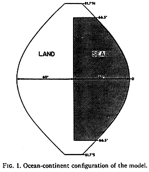
However, the computing time needed to model the ocean elements is considerable and truly tests their Univac 1108 computer. It takes 1,100 hours (about 46 days) to do just one run of the model. They are forced to use a highly simplified view of “Earth”, where a globe is split into three sections, equal parts ocean and land, with the poles omitted. Their paper (pdf) is published in the Journal of the Atmospheric Sciences and entitled, “Climate calculations with a combined ocean-atmosphere model”. July 1970 Study of Critical Environmental Problems
Williams College, Massachusetts. Credit: Daderot / Wikimedia Commons
More than 100 scientists and various experts from 17 US universities gather for a month-long meeting at Williamstown, Massachusetts, to discuss the “global climatic and ecological effects of man's activities”. The meeting results in a report published by the Massachusetts Institute of Technology in October of that year called the Study of Critical Environmental Problems (SCEP).
The report is criticised as being too US-centric and a follow-up, three-week meeting involving participants from 14 countries is organised in Stockholm in 1971. The resulting output is called “Inadvertent Climate Modification: Report of the Study of Man’s Impact on Climate” (SMIC).
Joseph Smagorinsky attends both meetings. Suki Manabe and Mikhail Budyko attend the SMIC meeting. The climate change working group at both meetings is led by NCAR’s William Kellogg. Global climate models are presented as being “indispensable” for researching human-caused climate change.
The SCEP and SMIC reports both influence the landmark June 1972 meeting, also held in Stockholm, called the United Nations Conference on the Human Environment, which leads to the founding of the UN Environment Program. Human-caused climate change is now on the radar of politicians. October 3, 1970 NOAA
With the support of President Richard Nixon, a “wet NASA” is created. It is called the National Oceanic and Atmospheric Administration, or NOAA, and sits within the US Department of Commerce. Nixon says it should “serve a national need for better protection of life and property from natural hazards…for a better understanding of the total environment”. This reflects a burgeoning interest – and concern – at this time about the way humans are impacting the environment. NOAA becomes one of the world’s leading centres of climate change research, with GFDL at Princeton being one of its key research centres.
October 1972 Met Office climate model
George Corby. Credit: G. A. Corby/Met Office
UK Met Office scientists describe in a journal paper the workings of their first GCM, which they’ve been developing since 1963 when the Met Office first created its “Dynamical Climatology Branch”. They write in the abstract: “The model incorporates the hydrological cycle, topography, a simple scheme for the radiative exchanges and arrangements for the simulation of deep free convection (sub grid-scale) and for the representation of exchanges of momentum, sensible and latent heat with the underlying surface.”
Using the UK-based ATLAS computer (considered at the time to be the world’s fastest supercomputer), the team, led by George Corby, use their five-layer model to show in a follow-up paper in 1973 that “despite the deterioration in the upper part of the model, reasonable simulation was achieved of many tropospheric features…There were also, however, a number of things that were definitely incorrect.”
The Met Office becomes one of the world’s leading centres of climate modelling in the decades ahead.
Manabe and Weatherald, 1975. Journal of the Atmospheric Sciences
January 1, 1975 Doubling of CO2
Manabe and Wetherald publish another seminal paper in the Journal of the Atmospheric Sciences, entitled “The Effects of Doubling the CO2 Concentration on the climate of a General Circulation Model”. They use a 3D GCM to investigate for the first time the effects of doubling atmospheric CO2 levels. The results reveal, among other things, disproportionate warming at the poles and a “significantly” increased intensity of the hydrologic cycle. It also shows a value for climate sensitivity of 2.9C – which is still, broadly, the mid-range consensus among climate scientists.
Manabe, Bryan and Spelman, 1975. Journal of Physical Oceanography
January 1, 1975 First coupled ocean-atmosphere GCM
At the same time as his paper with Wetherald, Manabe publishes a separate paper with Kirk Bryan. It presents the results from the first coupled atmosphere-ocean GCM (AOGCM). They say that, unlike their 1969 paper, it includes “realistic rather than idealized topography”. But it is still crude by today’s standards with a grid size of 500km. It takes 50 days of computing to simulate three centuries of atmospheric and oceanic interactions. “The climate that emerges from this integration includes some of the basic features of the actual climate,” they state. It correctly models areas of the world typified by extensive desert or high rainfall.
The paper is entitled, “A Global Ocean-Atmosphere Climate Model. Part I. The Atmospheric Circulation” and published by the Journal of Physical Oceanography. 1975 Understanding Climatic Change: A Program for Action
Understanding Climatic Change - A Program for Action. National Academy of Sciences
The National Academy of Sciences publishes a 270-page report by the US Committee for the Global Atmospheric Research Program (GARP) entitled, “Understanding Climatic Change: A Program for Action”. The committee has a number of notable names, including Charney, Manabe, Mintz, Washington and Smagorinsky. (It also includes Wally Broecker, whose 1975 Science paper first coined the term “global warming”, and Richard Lindzen, who would later become one of the most prominent climate sceptics.)
GARP had been tasked in 1972 with producing a plan for how best to respond to the increasing realisation that “man’s activities may be changing the climate”. GARP “strongly recommends” that a “major new program of research”, with “appropriate international coordination”, is needed to “increase our understanding of climatic change and to lay the foundation for its prediction”. To support this, it also recommends the development of a “wide variety” of models, accepting that realistic climate models "may be considered to have begun”.
Layers of Earth's atmosphere. Credit: Stocktrek Images, Inc. / Alamy Stock Photo
February 1977 Modelling methodologies published
A journal called Methods in Computational Physics: Advances in Research and Applications publishes an influential special volume on the “General Circulation Models of the Atmosphere”. Various climate modelling groups, including those at UCLA, NCAR and the UK Met Office, submit papers setting out how their current models work. Their papers – particularly the UCLA paper by Akio Arakawa and Vivian Lamb – form the backbone of most climate models’ “computational domain” for years afterwards.
Ad Hoc Study Group on Carbon Dioxide and Climate. National Academy of Sciences, 1979
July 23, 1979 — July 27, 1979 The Charney Report
The US National Research Council convenes a five-day “ad hoc study group on carbon dioxide and climate” at Woods Hole, Massachusetts. Chaired by Jule Charney, the assembled panel of experts (which includes a retired representative from the Mobil oil company) sets about establishing a “consensus” position on the “implications of increasing carbon dioxide”. To help them do so, they compare two models – one of Manabe’s and one by James Hansen at NASA’s Goddard Institute for Space Studies. The panel notes how heat from the atmosphere could be temporarily absorbed by the oceans and they also settle on a range for climate sensitivity of 2-4.5C, which has stayed largely the same ever since. 1980 World Climate Research Programme
The International Council of Scientific Unions and the World Meteorological Organization unite to sponsor the launch of the World Climate Research Programme (WCRP). Its main objective is “to determine the predictability of climate and to determine the effect of human activities on climate”. WCRP, which is based in Geneva, helps to organise observational and modelling projects at an international scale. Within a few years, its work helps to establish the understanding and prediction of El Niño and its associated impact on the global climate. It also leads to much better quality data collection of oceans which, in turn, helps climate modellers. 1983 Community Climate Model
NCAR’s Stephen Schneider and William Kellogg talking about climate models in a 1981 TV documentary.
The Community Climate Model (CCM) is created by the US National Center for Atmospheric Research (NCAR) in Colorado. It aims to be a “freely available global atmosphere model for use by the wider climate research community”. Its establishment recognises that climate models are getting increasingly complex and now involve the specific skills and inputs of a range of people. All of the source codes for the CCM (a 3D global atmospheric model) are published, along with a “users' guide”. A range of international partners are invited to take part, including the European Centre for Medium-Range Weather Forecasts.
Projecting the climatic effects of increasing carbon dioxide. United States Department of Energy, Dec 1985
December 1985 US Department of Energy report
The US government decides that it is “important to take an account” of how much climate science has moved on since the mid-1970s. So the Department of Energy commissions four “state of the art” volumes, which are reviewed by the American Association for the Advancement of Science. One of the volumes focuses on “projections”, in particular the “current knowns, unknowns, and uncertainties”. One area of focus is the “controversy” that “arose in 1979” when a paper (pdf) co-authored by MIT’s Reginald Newell concluded that climate models were overestimating climate sensitivity. Newell estimated a value lower than 0.25C.
The volume concludes: “Although papers continue to be published indicating order-of-magnitude shortcomings of model results, when these arguments have been carefully considered, they have been found to be based on improper assumptions or incorrect interpretations. Although the models are by no means perfect, where it has generally been possible to compare large-scale results from model simulations with measurements, the agreement has been good.”
Hansen et al, Journal of Geophysical Research, 1988
August 20, 1988 Hansen’s three scenarios
James Hansen is the lead author on a paper in the Journal of Geophysical Research: Atmospheres which examines various scenarios using a NASA GISS 3D model. They attempt “to simulate the global climate effects of time-dependent variations of atmospheric trace gases and aerosols”. They do this by running three scenarios in the model for the 30-year period between 1958 and 1988 and then see how this affects the modelled global climate up to 2060. The first scenario “assumes continued exponential trace gas growth” and projects 4C of warming by 2060 above 1958 levels.
Two months earlier, Hansen includes the paper’s finding in his now-famous US Senate hearing where he explains that human-caused global warming “is already happening now”. 1988 was, at that time, the warmest year on record.
Bert Bolin. Credit: KVA
November 1988 IPCC established
The United Nations Environment Programme (UNEP) and the World Meteorological Organization (WMO) establish the Intergovernmental Panel on Climate Change (IPCC). It becomes the leading international body for publishing periodic assessments of climate change. Its aim is to “provide the world with a clear scientific view on the current state of knowledge in climate change and its potential environmental and socio-economic impacts”. The first IPCC chair is Bert Bolin, a Swedish meteorologist, who had spent a year in 1950 working towards his doctorate at Princeton running early models on ENIAC, alongside the likes of Jule Charney and John von Neumann.
1989 The Atmospheric Model Intercomparison Project launches
Lawrence Livermore National Laboratory. Credit: National Ignition Facility / Wikimedia Commons
Under the auspices of the World Climate Research Programme, the Atmospheric Model Intercomparison Project (AMIP) is launched to establish a protocol that can be used to undertake the “systematic validation, diagnosis, and intercomparison” of all atmospheric GCMs. To do this, all models are required to simulate the evolution of the climate during the period 1979-88, according to standardised metrics.
AMIP is centred at the Program for Climate Model Diagnosis and Intercomparison at the Lawrence Livermore National Laboratory in California, but is a genuinely international attempt to standardise the assessment of the world’s various climate models. June 1989 New AOGCMs
Ronald Stouffer. Credit: John Mitchell
Around the same time, two modelling centres in the US start to publish results from their next-generation coupled atmosphere–ocean general circulation models (AOGCMs). At NCAR, Warren Washington and his colleague Gerald Meehl publish a paper in Climate Dynamics which uses their AOGCM to show how rising CO2 levels at three different rates affect global temperatures over the next 30 years.
Five months later, a paper in Nature by a team at the Geophysical Fluid Dynamics Laboratory at Princeton (led by Ronald Stouffer, but including Manabe and Bryan) sets out their AOGCM results, which highlight “a marked and unexpected interhemispheric asymmetry”. It concludes: “In the Northern Hemisphere of the model, the warming of surface air is faster and increases with latitude, with the exception of the northern North Atlantic.”
Margaret Thatcher opens the Met Office Hadley Centre. Credit: Met Office
May 25, 1990 Met Office Hadley Centre opens
Margaret Thatcher, the UK prime minister, formally opens the Met Office’s Hadley Centre for Climate Prediction and Research in Bracknell, Berkshire. Its strategic aims include “to understand the processes influencing climate change and to develop climate models”.
The first Hadley Centre coupled model boasts “11 atmospheric levels, 17 ocean levels and 2.5° × 3.75° resolution”. The Hadley Centre, now located in Exeter, remains to this day one of the world’s leading climate modelling centres.
August 27, 1990 — August 30, 1990 First IPCC report
First IPCC report. Credit: IPCC
At a meeting in Sweden, the IPCC formally adopts and publishes its first assessment report. Its summary of the latest climate model projections states that “under the IPCC business-as-usual emissions of greenhouse gases, the average rate of increase of global mean temperature during the next century is estimated to be about 0.3C per decade”.
The report carefully explains: “The most highly developed tool which we have to predict future climate is known as a general circulation model or GCM. These models are based on the laws of physics.” It says it has confidence in the models because “their simulation of present climate is generally realistic on large scales”.
But there’s a note of caution: “Although the models so far are of relatively coarse resolution, the large scale structures of the ocean and the atmosphere can be simulated with some skill. However, the coupling of [these] models reveals a strong sensitivity to small-scale errors which leads to a drift away from the observed climate. As yet, these errors must be removed by adjustments to the exchange of heat between ocean and atmosphere.”
September 20, 1990 Clouds
Credit: Unsplash
The Journal of Geophysical Research publishes an important paper (pdf) confirming that clouds are the main reason for the large differences – a “roughly threefold variation” – in the way the various models respond to changes in CO2 concentrations. Robert D Cess of Stony Brook University in New York and his co-authors (which include Wetherald, Washington and the Met Office’s John Mitchell) compare the climate feedback processes in 19 atmospheric GCMs.
They say their paper “emphasises the need for improvements in the treatment of clouds in these models if they are ultimately to be used as reliable climate predictors”. It follows a similar paper by Cess et al published a year earlier in Science. Together, the papers illustrate how climate scientists from across many countries are now working collectively to improve and refine their models. Clouds remain to this day a challenge for climate modellers. June 15, 1991 Eruption of Mount Pinatubo
Mount Pinatubo erupts, Luzon, Philippines. Credit: David Hodges / Alamy Stock Photo
A volcanic eruption in the Philippines – the second largest of the 20th century – provides a golden opportunity for scientists to further test climate models. Later that year, James Hansen submits a paper to Geophysical Research Letters which uses a NASA GISS climate model to forecast a “dramatic but temporary break in recent global warming trends”.
Over the coming years, climate models show that they can indeed accurately predict what impact the aerosols thrown into the atmosphere by Mount Pinatubo and other large volcanic eruptions can have, with the model results closely matching the observed brief period of global cooling post-eruption.
Image: Richinpit/E+/Getty Images
January 1992 Climate System Modeling' published
Cambridge University Press publishes a book called "Climate System Modeling", edited by NCAR’s Kevin Trenberth. The book is the end result of a series of workshops where scientists from a range of backgrounds – geography, physics, oceanography, meteorology, biology, public policy, etc – came together to set down the current knowledge about climate models. With 23 chapters written by 28 authors spreading over almost 800 pages, the book proves to be a vital reference. 1995 CMIP launched
Building on the development and success of AMIP in 1989, the World Climate Research Programme (WCRP) initiates the Coupled Model Intercomparison Project (CMIP). It aims to create a “standard experimental protocol” for studying the output of coupled atmosphere-ocean GCMs (AOGCMs) and, in particular, how they project climate change in the decades ahead.
The global community of modellers use CMIP to perform "control runs" where the climate forcing is held constant. In total, 18 models from 14 modelling groups are included. They compare how the various models “output” an idealised scenario of global warming, with atmospheric CO2 increasing at the rate of 1% per year until it doubles at about Year 70.
CMIP, which is currently on its sixth iteration, is still a bedrock of climate modelling today. August 10, 1995 Aerosols
Fig 4 from John Mitchell's paper. Credit: Mitchell et al/Nature
John Mitchell at the Met Office is the lead author of a much-cited paper in Nature which – for the first time in a GCM – tests what impact including sulphate aerosols has on the radiative forcing of the atmosphere. The authors find that their inclusion “significantly improves the agreement with observed global mean and large-scale patterns of temperature in recent decades” and leads them to a striking conclusion: “These model results suggest that global warming could accelerate as greenhouse-gas forcing begins to dominate over sulphate aerosol forcing.”
Mitchell’s paper builds on earlier work showing how rising quantities of aerosols might affect radiative forcing. For example, Science had published a much-discussed paper in 1971 by Ichtiaque Rasool and Stephen Schneider, both then at NASA GISS, entitled “Atmospheric carbon dioxide and aerosols: Effects of large increases on global climate”. It concluded: “An increase by only a factor of 4 in global aerosol background concentration may be sufficient to reduce the surface temperature by as much as 3.5K. If sustained over a period of several years, such a temperature decrease over the whole globe is believed to be sufficient to trigger an ice age.” September 10, 1995 Draft of IPCC’s second assessment report The New York Times reports that it has obtained a draft of the IPCC’s second report. The newspaper says the IPCC, in “an important shift of scientific judgment”, has concluded that “human activity is a likely cause of the warming of the global atmosphere”.
However, much of the newspapers’ focus is on the IPCC’s assessment of the accuracy of climate models’ projections: “The models have many imperfections, but the panel scientists say they have improved and are being used more effectively.”
The paper notes that the scientists’ confidence has been “boosted by more powerful statistical techniques used to validate the comparison between model predictions and observations”. However, it says “despite the new consensus among panel scientists, some skeptics, like Dr Richard S Lindzen of the Massachusetts Institute of Technology, remain unconvinced”. Lindzen is quoted as saying that IPCC's identification of the greenhouse signal "depends on the model estimate of natural variability being correct". Models do not reflect this well, he says.
Credit: US Government Printing Office, archive.org
November 16, 1995
November 16, 1995 US Congressional hearing into climate models
At the US Congress in Washington DC, the House Subcommittee on Energy and Environment holds a hearing into “climate models and projections of potential impacts of global climate change”. It is part of a wider inquiry into the “integrity and public trust of the science behind federal policies and mandates”. It is chaired by Dana Rohrabacher, a Republican congressman who goes on to become a prominent climate sceptic politician in the US.
A “balance” of expert witnesses is called to give evidence. They include the climate sceptic Pat Michaels and UK climate scientist Bob Watson, who later becomes the IPCC chair. Rohrabacher says he wants to “promote dialogue” among the witnesses due to the “controversy” over the “reliability” of climate models. He asks: “Are we so certain about the future climate changes that we should take action that will change the lives of millions of our own citizens at a cost of untold billions of dollars?”
The event sets the tone and template for many other similar hearings on the Hill in the years ahead.
July 4, 1996 Santer’s ‘fingerprint’ study
Ben Santer in the film Merchants of Doubt, 2014. Credit: Everett Collection Inc / Alamy Stock Photo
Ben Santer is the lead author of an influential paper in Nature which shows that “state-of-the-art models” match the “observed spatial patterns of temperature change in the free atmosphere from 1963 to 1987” when various combinations of changes in greenhouse gases and aerosols are added. They concluded from their modelling that “it is likely that this trend is partially due to human activities, although many uncertainties remain, particularly relating to estimates of natural variability”.
This attribution study – sometimes called a “fingerprint” study – comes just months after the IPCC’s second assessment report had concluded that “the balance of evidence suggests that there is a discernible human influence on global climate”. Santer had been a key author for the chapter that shaped that wording. That statement – and Santer et al’s Nature paper – are both aggressively attacked by climate sceptics, but later substantiated by scientists. March 15, 2000 IPCC’s Special Report on Emissions Scenarios
Professor Nebojsa Nakicenovic. Credit: Silveri/IIASA
By the end of the 1990s, climate modellers are starting to work much more closely with integrated assessment modellers to help produce projections that are more relevant to policymakers eager to find the least-cost pathways to reducing emissions.
In 2000, the IPCC publishes a special report on emissions scenarios (SRES): “They include improved emission baselines and latest information on economic restructuring throughout the world, examine different rates and trends in technological change and expand the range of different economic-development pathways, including narrowing of the income gap between developed and developing countries.”
The IPCC team is led by Nebojsa Nakicenovic of the International Institute for Applied Systems Analysis (IIASA) in Austria. The SRES are used for the IPCC’s third assessment report in 2001, but are later further developed into the Representative Concentration Pathways (RCPs) in time for the IPCC’s fifth assessment report in 2014. November 9, 2000 Carbon cycle included in climate models
A team of UK-based climate scientists, led by Peter Cox at the Met Office, publish in Nature the results from the first “fully coupled three-dimensional carbon-climate model”. They conclude that carbon-cycle feedbacks could “significantly accelerate” climate change over the course of the 21st century: “We find that under a ‘business as usual’ scenario, the terrestrial biosphere acts as an overall carbon sink until about 2050, but turns into a source thereafter.”
The scientists couple a dynamic global vegetation model – called “TRIFFID” – with an ocean-atmosphere model and an ocean carbon-cycle model. Adding TRIFFID means that soil carbon and “five functional types” of plant (“broadleaf tree, needleleaf tree, C3 grass, C4 grass and shrub”) are included in climate models for the first time. October 5, 2004 ‘Extreme event’ attribution study
Summer heatwave in Paris. Credit: Idealink Photography/ Alamy Stock Photo
Following the deadly European heatwave in 2003, two UK-based climate scientists, Peter Stott and Myles Allen, publish a paper (pdf) in Nature showing that it was “very likely” that “human influence” at least doubled the chances of it occurring.
Stott and Allen do not try to establish whether human-caused emissions “caused” the extreme heatwave. Rather, they use modelling to show probabilistically that emissions raised the chances of the heatwave occuring. The paper triggers many more extreme event attribution studies, many of which are performed in near-realtime so the results can be published days after the actual event. December 5, 2007 Santer vs Douglass
University of Rochester. Credit: Peter Steiner/Alamy Stock Photo
The International Journal of Climatology publishes a paper by a team of climate sceptic scientists, led by David H Douglass at the University of Rochester, which compares “tropospheric temperature trends of 67 runs from 22 ‘Climate of the 20th Century’ model simulations” with observed temperature trends in the tropical troposphere. They argue that there is “disagreement” between the two, “separated by more than twice the uncertainty of the model mean”. The results attract a lot of media attention.
Ten months later, a diverse group of climate modellers, led by Ben Santer, publish a paper in response in the same journal. It concludes: “This claim was based on use of older radiosonde and satellite datasets, and on two methodological errors: the neglect of observational trend uncertainties introduced by interannual climate variability, and application of an inappropriate statistical ‘consistency test’.”
Santer and his colleagues then become the focus of a coordinated campaign, which includes repeated freedom of information requests for their code, emails and data. The episode is further inflamed by the “Climategate” affair in 2009, when stolen emails sent by climate scientists are selectively quoted by climate sceptics and media in an attempt to undermine climate science.
The “Santer vs Douglass” episode typifies the way climate sceptics have sought to undermine and criticise climate modelling since at least the early 1990s. February 12, 2008 Tipping elements
A collapsing ice shelf - Larsen B in 2005. Credit: NASA Earth Observatory
A team of scientists led by Tim Lenton at the University of East Anglia publish a paper in PNAS which uses climate models and palaeoclimate data to explore climatic “tipping points” - or tipping elements, as they call them – in response to rising human-caused emissions.
The paper lists six tipping elements it believes are of “policy relevance”, should emissions continue to rise: reorganisation of the Atlantic thermohaline circulation; melting of the Greenland ice sheet; disintegration of the West Antarctic ice sheet; Amazon rainforest dieback; dieback of boreal forests; and shift of the El Niño-Southern Oscillation regime to an El Niño-like mean state.
The paper offers a stark conclusion: “Society may be lulled into a false sense of security by smooth projections of global change. Our synthesis of present knowledge suggests that a variety of tipping elements could reach their critical point within this century under anthropogenic climate change. The greatest threats are tipping the Arctic sea-ice and the Greenland ice sheet.” March 23, 2008 Black carbon
Flames leak from a gas/oil pipe on the edge of the Sahara desert, Libya. Credit: Purple Pilchards / Alamy Stock Photo
Nature publishes a paper by two US-based scientists, Veerabhadran Ramanathan and Greg Carmichael, which examines the “dimming” influence of “black carbon” on the atmosphere. Black carbon is the term for sooty aerosols thrown into the atmosphere through the burning of fuels, such as coal, diesel, wood and dung. The paper also examines how “the deposition of black carbon darkens snow and ice surfaces, which can contribute to melting, in particular of Arctic sea ice”.
“Aerosols in aggregate are either acting to, you could say, cool the atmosphere or mask the effect of CO2,” Carmichael tells the Guardian. “[Black carbon] is the only component of this aerosol mix that in and of itself is a heating element.” The authors argue that the impact of black carbon has, to date, been underestimated by the models. September 22, 2008 — September 24, 2008 CMIP5
After four phases of the Coupled Model Intercomparison Project (CMIP), 20 climate modelling groups from around the world gather for a meeting at the Ecole Normale Superiéure in Paris to discuss the fifth phase. They agree to a new set of climate model experiments which aim to address outstanding questions that arose from the IPCC’s fourth assessment report published the year before. CMIP5 becomes the foundational set of coordinated modelling experiments used for the IPCC fifth assessment report published in 2013.
CMIP5 includes decadal predictions (both hindcasts and projections), coupled carbon/climate model simulations, as well as several diagnostic experiments used for understanding longer-term simulations out to 2100 and beyond. September 7, 2012 A National Strategy for Advancing Climate Modeling
NASA's visualisation of CO2 emissions in 2006. Credit: NASA
In the US, the National Research Council publishes a “National Strategy for Advancing Climate Modeling”. The report recognises that evolutionary changes to computing hardware and software present a challenge to climate modellers: “Indications are that future increases in computing power will be achieved not through developing faster computer chips, but by connecting far more computer chips in parallel – a very different hardware infrastructure than the one currently in use. It will take significant effort to ensure that climate modeling software is compatible with this new hardware.” To date, the recommendations have largely not been delivered. September 23, 2013 — September 27, 2013 IPCC’s fifth assessment report
Stockholm, Sweden, 2013. Credit: Arseniy Rogov/Alamy Stock Photo
At a meeting in Stockholm, Sweden, the IPCC publishes the first report of its fifth assessment cycle (AR5). The report includes an evaluation of the models. It concludes: “The long-term climate model simulations show a trend in global average surface temperature from 1951 to 2012 that agrees with the observed trend (very high confidence). There are, however, differences between simulated and observed trends over periods as short as 10 to 15 years (eg, 1998 to 2012).”
This recent “observed reduction in surface warming trend” – sometimes labelled as a “slowdown” or, inaccurately, as a “pause” or “hiatus” – subsequently becomes a focus of study for climate modellers. Four years later, a paper published in Nature in 2017 seeks to “reconcile the controversies” and concludes that a “combination of changes in forcing, uptake of heat by the oceans, natural variability and incomplete observational coverage” were to blame. The authors state that, as a result of their findings, “we are now more confident than ever that human influence is dominant in long-term warming”.
Reflecting new understanding of radiative forcings, AR5 also slightly adjusts the IPCC’s range of equilibrium climate sensitivity to “1.5C to 4.5C (high confidence)”. It adds: “The lower temperature limit of the assessed likely range is thus less than the 2C in the AR4, but the upper limit is the same.” October 6, 2017 — October 10, 2017 IPCC’s sixth assessment report
Valerie Masson-Delmotte, co-chair of Working Group I, at the 46th Session of the Intergovernmental Panel on Climate Change, 6 September 2017.
Climate scientists gathered in Montreal for the IPCC’s annual meeting agree to the chapter outline for AR6, which is due to be published in parts over a few months in 2021-22. The working group one report will include various “evaluations” of how the models have developed and performed since AR5. It will incorporate modelling results from the sixth cycle of CMIP, as well as an extended set of RCP scenarios. Each RCP will be paired with one or more “Shared Socioeconomic Pathways”, or SSPs, which describe potential narratives of how the future might unfold in terms of socioeconomic, demographic and technological trends.